6 Methods
6.1 Study Area
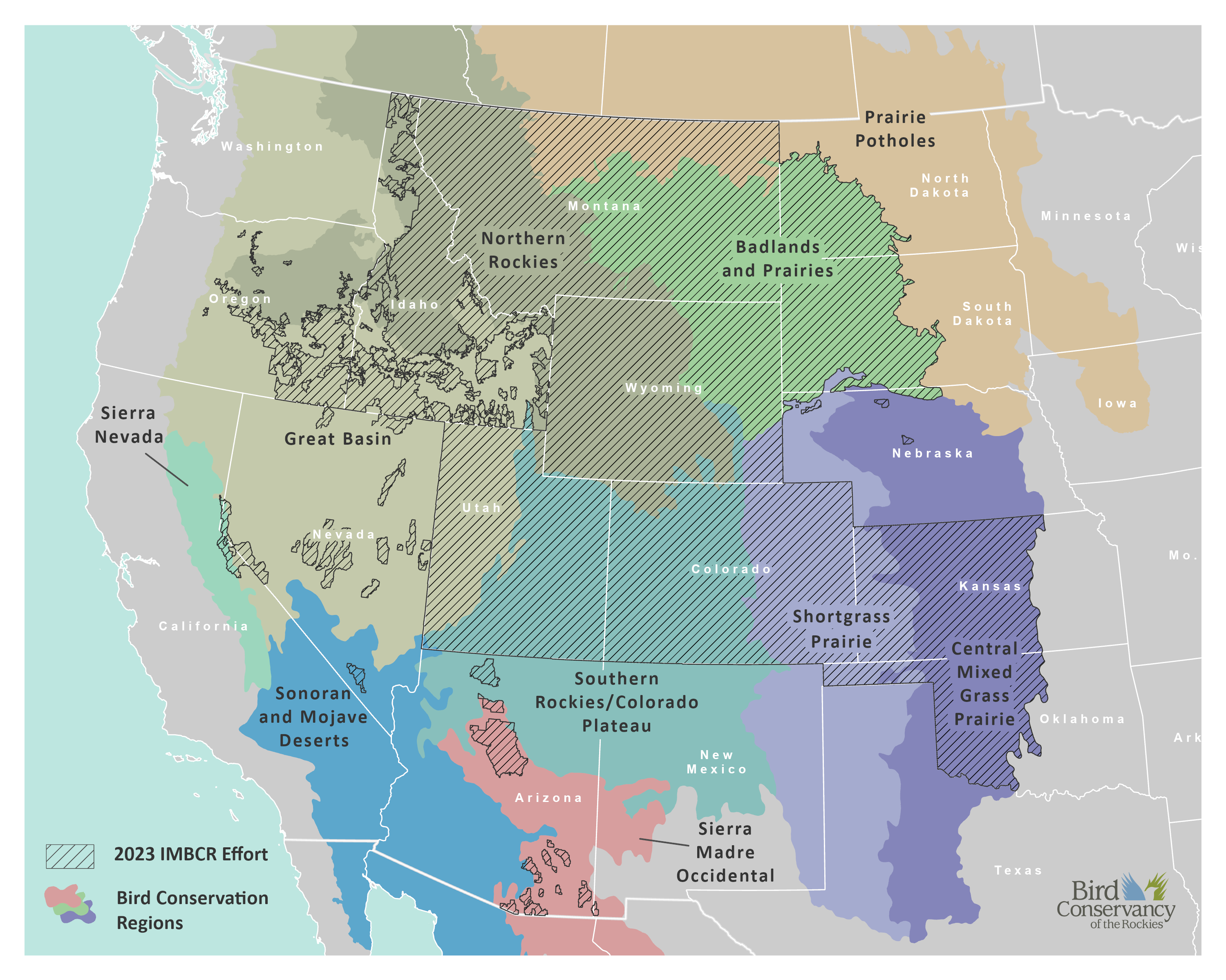
In 2023, the IMBCR program’s area of inference encompassed four entire states (Colorado, Montana, Utah, and Wyoming) and portions of 11 additional states (Arizona, California, Idaho, Kansas, Nebraska, Nevada, New Mexico, North Dakota, Oklahoma, Oregon, and South Dakota). We surveyed across US Forest Service (USFS) Regions 1, 2, and 4 and in portions of Region 3; all of the Badlands and Prairies Bird Conservation Region (BCR 17), and portions of nine other BCRs: Great Basin (9), Northern Rockies (10), Prairie Potholes (11), Sierra Nevada (15), Southern Rockies/Colorado Plateau (16), Shortgrass Prairie (18), Central Mixed Grass Prairie (19), Sonoran and Mojave Deserts (33), and Sierra Madre Occidental (34).
6.2 Sampling Design
Sampling Frame and Stratification
A key feature of the IMBCR design is the ability to estimate bird population parameters at multiple spatial scales, from small management units, such as individual national forests or field offices, to entire states and BCRs. This is accomplished through hierarchical (nested) sampling of smaller within larger units. The fundamental units of the design (and therefore of population estimation) are strata, which are mutually exclusive and together form the programmatic footprint in any given year. Strata-level population estimates can be combined to derive estimates at larger scales for groups of strata (hereafter superstrata). For example, data from each individual national forest stratum in USFS Region 2 are combined to produce Region-wide population estimates; data from each individual stratum in Montana are combined to produce statewide estimates; and data from each individual stratum in BCR 17 are combined to produce BCR-wide estimates.
We define strata based on areas to which IMBCR partners wanted to make inferences. Strata contributing to the baseline monitoring effort (hereafter background strata) are nested within the intersection of state and BCR boundaries (e.g., Wyoming-BCR 10). Additionally, we base background strata within the state-BCR sampling frames on fixed attributes, such as land ownership boundaries, elevation zones, major river systems and wilderness/roadless designations. Additional strata defined for particular objectives, such as monitoring within areas subject to management action, are not subject to the same constraints as background strata (hereafter overlay strata).
Sampling Units
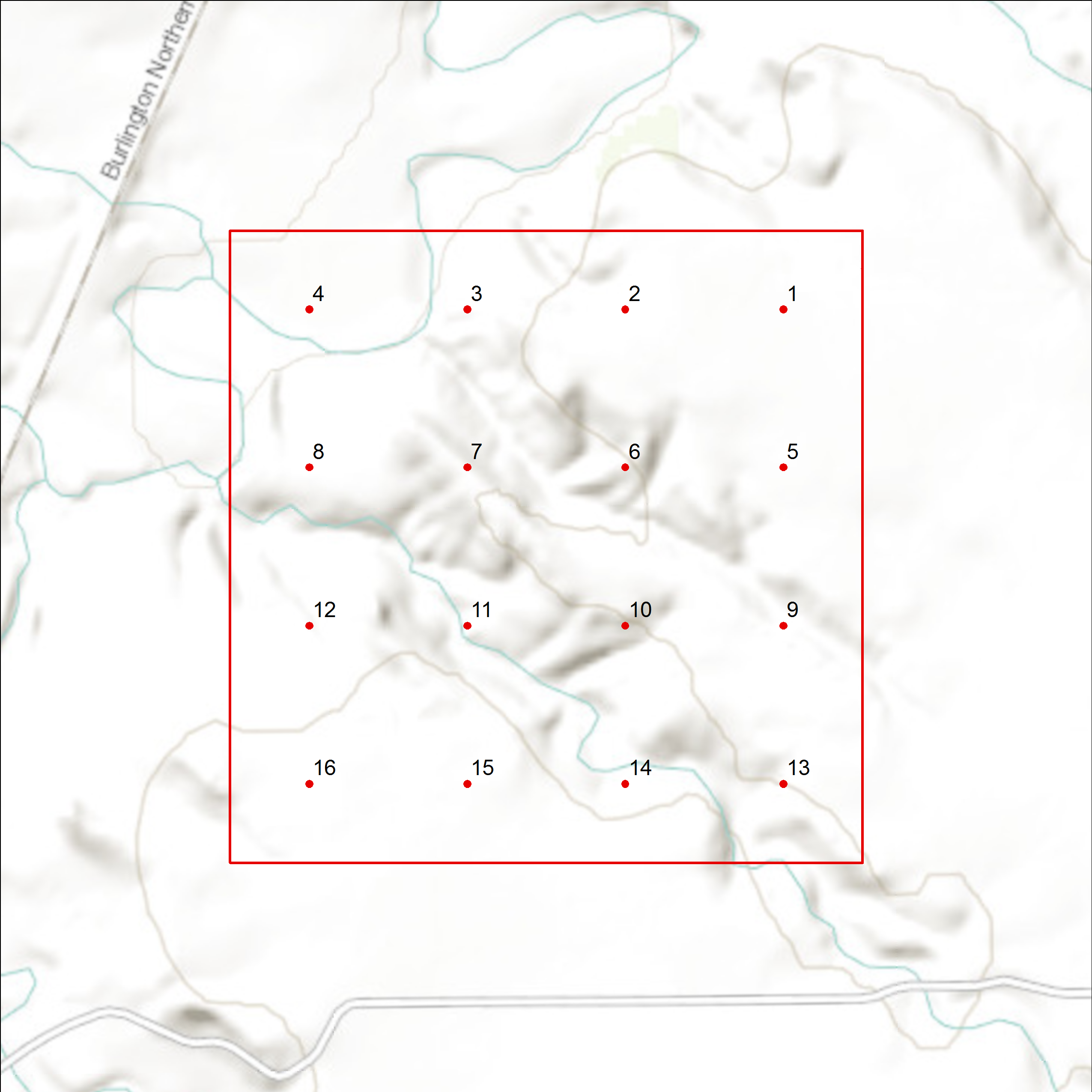
We define sampling units as 1 km² cells, each containing 16 evenly spaced sample points, 250 meters apart (Figure 6.2). We define potential sampling units by superimposing a uniform grid of cells over each state in the study area. We then assign each cell to a stratum using ArcGIS version 10.X and higher (Environmental Systems Research Institute, 2017). For all stratifications developed after 2012, we use the United States National Grid (USNG), a nonproprietary alphanumeric referencing system derived from the Military Grid Reference System that was created by the Federal Geographic Data Committee.
Sample Selection
Within each stratum, we use generalized random-tessellation stratification (GRTS), a spatially balanced sampling algorithm, to select sampling units (Stevens Jr. & Olsen, 2004). The GRTS design has useful properties with respect to long-term monitoring of birds at large spatial scales including:
Spatially balanced sampling is generally more efficient than simple random sampling of natural resources (Stevens Jr. & Olsen, 2004). Incorporating information about spatial autocorrelation in the data can increase precision in density estimates.
All sampling units in the sampling frame are ordered, such that any set of consecutively numbered units is a spatially well-balanced sample (Stevens Jr. & Olsen, 2004). In the case of fluctuating budgets, IMBCR partners can adjust the sampling effort among years within each stratum while still preserving a random, spatially balanced sampling design.
We require two sampling units to be surveyed within each stratum, but reliable stratum-level occupancy estimates require larger sample sizes, with a minimum of approximately 8-10 samples per stratum. Additional samples may be required for strata comprising large geographic areas. Because we estimate regional density and occupancy using an area weighted mean, adding more samples to a particular stratum does not bias the overall estimate, it simply increases the precision. After the initial two sampling units were selected, the remaining allocation of sampling effort among strata was based on the priorities of the funding partners.
6.3 Sampling Methods
IMBCR observers with excellent aural and visual bird-identification skills conducted field work in 2022. Prior to conducting surveys, observers completed an intensive training program to ensure full understanding of the field protocol and review bird and plant identification. Observers were also shadowed by a crew leader at the start of the field season to ensure they understood the protocol and could identify all birds within a region.
Observers conducted point counts (Buckland et al., 2001) following protocols established by IMBCR partners (Hanni, White, Birek, Van Lanen, & McLaren, 2012). Observers conducted surveys in the morning, beginning one-half hour before sunrise and concluding no later than five hours after sunrise. Observers recorded the start time for every point count conducted. For every bird detected during the six-minute period, observers recorded species, sex, horizontal distance from the observer, minute, type of detection (e.g., call, song, visual), whether the bird was thought to be a migrant, and whether the observer was able to visually identify each record.
Observers measured distances to each bird using laser rangefinders when possible. When it was not possible, observers estimated the distance by measuring to some object near the bird using a laser rangefinder. In addition to recording all bird species detected in the area during point counts, observers recorded birds flying over but not using the immediate surrounding landscape. Observers also recorded Abert’s squirrel (Sciurus aberti), American red squirrel (Tamiasciurus hudsonicus), and American pika (Ochotona princeps). While observers traveled between points within a sampling unit, they recorded the presence of any species not recorded during a point count. The opportunistic detections of these species are used for distribution purposes only.
Observers considered all non-independent detections of birds (i.e., flocks or pairs of conspecific birds together in close proximity) as part of a “cluster” rather than as independent observations. Observers recorded the number of birds detected within each cluster along with a letter code to distinguish between multiple clusters.
At the start and end of each survey, observers recorded time, ambient temperature, cloud cover, precipitation, and wind speed. Observers navigated to each point using hand-held Global Positioning System units. Before beginning each six-minute count, surveyors recorded vegetation data within a 50m radius of the point via ocular estimation. Vegetation data included the dominant habitat type and relative abundance, percent cover and mean height of trees and shrubs by species, grass height, and ground cover. Observers recorded vegetation data quietly to allow birds time to return to their normal habits prior to beginning each count.
For more detailed information about survey methods and vegetation data collection protocols, refer to Bird Conservancy’s Field Protocol for Spatially Balanced Sampling of Landbird Populations (contact Jennifer Timmer to request a copy.
6.4 Data Analysis
Framework and terminology
We applied hierarchical models using Bayesian tools to estimate abundance, density, occupancy, and their respective trends. Hereafter, we refer to abundance, density, and occupancy as “primary population parameters”, or simply “population parameters”, and estimates of these parameters as “population estimates”. Abundance is the number of species members present within a specified areal unit and time frame. Density is abundance per unit area (birds per \(km^2\)). Occupancy is the probability or proportion of sampling units within an areal unit and time frame where at least one species member is present. Because population estimates are derived from data collected over 6-min surveys conducted once per sampling period (i.e., the breeding season), the time frame of estimation is 6 minutes. Thus, IMBCR abundance and occupancy estimates quantify the number of individuals present and the proportion of sampling units (or area) with \(\geq1\) individual present, respectively, within a 6 minute snapshot in time. In contrast, other monitoring programs that estimate population parameters over longer time frames that allow movement into the sampling unit during the sampling period will tend to quantify the distribution of breeding territories or home ranges (i.e., space use; for further details, see Section D.1.5 in Appendix D).
Given our sampling design (see above), the fundamental areal unit of estimation for all parameters is the stratum, and so our models estimate abundance, density, and occupancy for all strata making up the IMBCR programmatic footprint. Additionally, our design allows us to derive population estimates for larger areal units consisting of \(\geq2\) strata (hereafter superstrata) by summarizing across component strata. For density and occupancy, superstrata estimates represent means of component strata weighted by their area. For abundance, we simply sum component strata estimates to derive superstrata estimates. Hereafter, we use the term “areal units” to refer to strata and superstrata in general. To allow flexible trend estimation for any areal unit and time period, trend estimation involves post hoc analysis of annual population estimates generated by a primary estimation model (Appendix D). Finally, analyzing data in a manner consistent with the IMBCR design, we leverage all available information across the IMBCR program to estimate parameters representing the observation process, which by extension improves precision of population estimates. For further details on the structure of our analysis models, see Appendix D.
Data filtering
We set minimum data thresholds applied to each species for estimating population parameters. We estimated abundance and occupancy for all species with \(\geq 30\) detections recorded across the IMBCR program. For species with 10-29 detections, we estimated only occupancy using occupancy models. For species with fewer detections, we did not attempt to estimate any population parameters. These criteria were applied after excluding the furthest 10% of detections following standard practice for distance sampling (see Section D.1.5 in Appendix D). Thus, in practice, the minimum number of detections required was 33 for estimating abundance.
For each species, we only analyzed data from strata where the species was detected at least once during at least one year. We thus conditioned strata-level estimation on the species having been detected at least once, thereby (conservatively) excluding strata outside the range of the species. When rolling up strata to superstrata estimates, we assumed surveyed strata that were thus excluded from primary strata-level estimation to have density and occupancy estimates of zero.
Model Assumptions
Distance sampling theory was developed to account for the decreasing probability of perceiving an object of interest (e.g., a bird) with increasing distance from the observer to the object (Buckland et al., 2001). Estimated perceptibility is used to adjust the count of birds to account for birds that were present but not perceived within sampled area. Application of distance theory requires that five critical assumptions be met: 1) all birds at and near the sampling location (distance = 0) are perceived; 2) distances to birds are measured accurately; 3) detected birds do not move in response to the observer’s presence prior to detection (Buckland et al., 2001; Thomas et al., 2010); 4) cluster sizes are recorded without error; and 5) the sampling units are representative of the entire survey region (Buckland, Marsden, & Green, 2008).
Starting in 2023, we added time-removal sampling to account for imperfect availability for perception. Imperfect availability can arise, for example, from birds being hidden from view and quiet during some portion of their daily activities. The addition of removal sampling data (i.e., the time period of detection within the 6 min survey) can be seen as relaxing assumption 1 (Amundson et al. 2016). Regardless, we now account for two components of detection probability, a spatial component accounting for distance from the surveyor and a temporal component accounting for incomplete availability for detection, theoretically improving accuracy of our population estimates over estimates prior to 2023, which only accounted for the former.